This project is taken from and is an extention of my master's dissertation which can be found here
|
MPC does not refer to any one algorithm or method but instead a methodological philosophy with which to approach control problems, containing certain key concepts and ideas implemented in various ways. There are 3 main components in a GPC algorithm: |
|
|
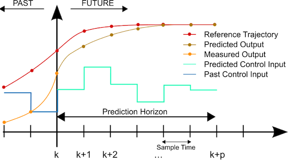
The prediction stage of a GPC algorithm uses the model to predict the future states of the system, if provided with some sequence of control actions. This is derived by recursively implementing the systems model unto itself to produce a higher order prediction model over a specified horizon length. Given a linear state space system, a state prediction model for a horizon of length N, and evaluated at a time instance k, can be defined as: |
i \begin{equation} \bar{X}(k) = F X(k) + G \bar{\mu}(k) \end{equation} \begin{equation} \bar{X}(k) = \begin{bmatrix} X(k+1|k)\\ X(k+2|k)\\ \vdots\\ X(k+N|k) \end{bmatrix} , \bar{\mu}(k) = \begin{bmatrix} \mu(k|k)\\ \mu(k+1|k)\\ \vdots\\ \mu(k+N-1|k) \end{bmatrix} , F = \begin{bmatrix} A_{dt}\\ A_{dt}^{2}\\ \vdots\\ A_{dt}^{N} \end{bmatrix} , G = \begin{bmatrix} B_{dt} & 0 & \dots & 0\\ A_{dt}B_{dt}& B_{dt}& \dots & 0\\ \vdots& \vdots & \ddots & \vdots\\ A_{dt}^{N-1}B_{dt}& A_{dt}^{N-2}B_{dt} & \dots & B_{dt} \end{bmatrix} \end{equation}
|
The Optimisation stage seeks to formulate and solve an optimisation problem \(P_N(X(0))\), to obtain the minimising control sequence over the whole horizon \(\bar{\mu}\), evaluated at each time step k, where: |
ii \begin{equation} min_\mu V_N(X(0),\bar{\mu}) = \sum_{i = 0}^{i = N-1} X^{T}(k+i|k) Q X(k+i|k) + \mu^{T}(k+i|k) R \mu(k+i|k) \end{equation} s.t \[ X(k|k) = X(k) \] \[ X(k+1+i|k) = A_{dt}X(k+i|k) + B_{dt} \mu(k+i|k) , i=1,2,3\dots,N-1 \]
|
Where \(Q^{n \times n}\), and \(R^{m \times m}\), are 2-norm weighing matrices on the states and inputs respectively. If equation i, is substituted into ii, this puts ii into the standard form of a quadratic programming problem where: |
iii \begin{equation} V_N(X(0),\bar{\mu}) = min_\mu \frac{1}{2} \bar{\mu}^{T}(k) H \bar{\mu}(k) + C_q^{T}\bar{\mu}(k) + \alpha \end{equation} \[H = 2(G + \tilde{Q}G + \tilde{R})\] \[C_q = L X(k) , L = 2 G^{T} \tilde{Q} F\] \begin{equation} \alpha = X(0)^{T} M X(0), M = F^{T} \tilde{Q} F + Q \end{equation}
|
With \( \tilde{Q} \) and \(\tilde{R}\) being \(N-1 \times N-1\) dimensional matrix diagonal matrices, with the Q and R matrices as diagonal terms respectively. Solving this Quadratic Program produces a 1 by mxN optimal control sequence where the optimal control gain, \(K_N\), consists of the first \(m \times n\) terms in \(-H^{-1} L\) due to the implementation of the receding horizon principle: |
\begin{equation} \bar{\mu }= -H^{-1} L X(k) \end{equation}
|
This is the reason MPC implementations are also known as receding horizon control (RHC) as they only perform the first set of control actions in the sequence \(\bar{\mu}\), before recalculating and performing this action at every time interval, k, until the target is reached. This continual updating provides feedback into the system. |
|