This project is taken from and is an extention of my master's dissertation which can be found here

Simulation and Linear Quadratic Guassian Control of Y-6 UAV

The purpose of designing and implementing control systems is to reject or minimise the effects of disturbance on systems, as well as change the characteristics of the system to meet performance requirements. Therefore in order to accomplish this with the UAV, LQG, LQ-MPC and PID control systems will be developed and the following themes will be explored:

Discretization
Analysis
LQG
LQ-MPC
PID

Discretization

The Linearised model obtained is derived in previous section is in the continuous-time domain. However, to design control systems which can be implemented unto digital computers, the control laws must be in the discrete-time domain. This can be done either by designing the control systems in the continuous-time domain then converting the resulting continuous control laws into discrete ones, or by transforming the entire continuous-time model to the discrete-time domain then designing the control laws using the discrete-time system model. This project utilises the latter method. To convert a continuous-time state space model of form:

$\dot{X (t)} = A X (t) + B μ (t)$

to the discrete-time domain Produces:

$X (k + 1) = A_{d t} X (k) + B_{d t} μ (k)$

where:

$A_{d t} = e^{A T}$ $B_{d t} = A^{- 1} (e^{A T} - I) B$

and T is the discretization sample time, k is the time increment, and I an identity matrix of sufficient dimension.

Analysis

Stability

Stability theory plays a key role in the design of control systems. There are different kinds of stability problems that arise in the study of dynamical systems. The stability of systems about equilibrium operating points is usually characterised in the Lyapunov sense where an equilibrium point is said to be stable if all solutions starting nearby the equilibrium points stay nearby for all time, otherwise the system is said to be unstable. This definition of stability can be further specified to define stability in the asymptotic sense, where a system is said to be asymptotically stable if all solutions starting nearby the equilibrium points not only stay nearby, but also tend to the equilibrium point as time goes to infinity. 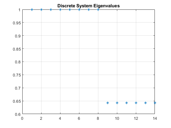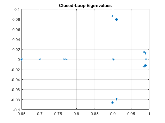For linear state-space systems, stability can be assertained from the locations of the eigenvalues, $λ$ , of the $A_{d t}$ matrix, This process is know as Lyapunov's indirect method.

$d e t | A_{d t} - λ I | = 0$

A look at the systems eigen values reveals the presence 6 eigenvalues with a value less than 1, and 8 eigenvalues with a value of 1. For discrete-time systems, stability can be said to be asymptotic if all eigenvalues are strictly within the unit circle, Lyapunov if all eigenvalues are within or on the unit circle, and unstable otherwise. Therefore the linear systems model can be said to be stable in the sense of Lyapunov. This implies also that the non-linear systems model is locally stable in the sense of Lyapunov about the equilibrium points $X_{e}$ . However due to real world disturbances such as model uncertainty, sensor noise and external wind disturbances, the system will not remain at the point of equilibrium save for the intervention of some control law to reject the effect of these disturbances. Hence, the system, although statically stable, is dynamically unstable.

Reachability

Reachability is a property which is determined by coupling between the inputs and the system states, a system is said to be reachable if for any initial set of state values $X_{0}$ , and any final set of state values, $X_{f}$ , there is a control signal $μ (k)$ that can take the system from $X_{0}$ at k = 0, to $X_{f}$ within some finite time. A system is said to be reachable if the reachability matrix is full rank equalling the number of state, n:

W_{r} = [\begin{matrix} B_{d t} & A_{d t} B_{d t} & \dots & A_{d t}^{n - 1} B_{d t} \end{matrix}]

Thus, as the rank of $W_{r}$ is equals to n, the system can be said to be reachable. The less stringent property of stabilisability can also be defined where only the unstable states need be reachable.

Observability

Observability is a property which is also determined by coupling, in this case, between the system outputs and states. Therefore the system outputs, $Y$ , must be defined where $Y$ is a subset of the state $X$ .

$Y = [z, ϕ, θ, ψ]$

$Y (k) = C X (k)$

$C = [\begin{matrix} 1 & 0 & 0 & 0 & 0 & 0 & 0 & 0 & 0 & 0 & 0 & 0 & 0 & 0 \\ 0 & 0 & 1 & 0 & 0 & 0 & 0 & 0 & 0 & 0 & 0 & 0 & 0 & 0 \\ 0 & 0 & 0 & 0 & 1 & 0 & 0 & 0 & 0 & 0 & 0 & 0 & 0 & 0 \\ 0 & 0 & 0 & 0 & 0 & 0 & 1 & 0 & 0 & 0 & 0 & 0 & 0 & 0 \end{matrix}]$

C \in R^{p = 4 \times n}

C_{d t} = C

A system is said to observable if for all time, it is possible to, from a limited set of state measurements $Y (k)$ , and knowledge of the inputs $μ (k)$ , uniquely obtain the full state, X(k). A system is said to be observable if the observability matrix is full rank equalling n:

$W_{o} = [\begin{matrix} C_{d t} \\ C_{d t} A_{d t} \\ ⋮ \\ C_{d t} A_{d t}^{n - 1} \end{matrix}]$

As with reachability, a less stringent property, detectability, can also be defined where only the unstable states need be observable.

Interestingly, for this combination of $A_{d t}$ and $C_{d t}$ , it is found that $W_{0}$ is not full rank, and therefore the system in its current form is not observable. Upon further analysis, it is discovered that this is as a result of the Coaxial propulsion unit configuration, as there are numerous combinations of thrust force values that each individual propulsion unit can generate which produce the same resultant torque about the centre of mass making it impossible to obtain a unique full state. One possible solution is to modify the UAV design to include RPM sensors to measure at least 2 non-coaxial motors. However, in the upcoming LQG subsection, a more elegant solution is proposed.

Linear Quadratic Gaussian Control (LQG)

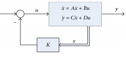
Full State Feedback

Full-state feedback is a control technique which makes use of the full-state, $X (k)$ of a system, to modify the system's eigenvalue so as to change its characteristic responses. This is done by determining some set of gains K which when applied to the system states, the resultant of which being fed back into the system as inputs, adjust the dynamics of the system, where:

$μ (k) = - K X (k)$

This leads to a modified closed loop system:

$X (k + 1) = (A_{d t} - B_{d t} K) X (k)$

Where the eigenvalues are now determined by:

$d e t | (A_{d t} - B_{d t} K) - λ I | = 0$

Linear Quadratic Regulator (LQR)

LQR is a technique for finding the set of gains K, in a manner which is in some wise optimal. In order to accomplish this, LQR seeks to find a control sequence $μ$ to minimise a quadratic cost function by formulating the control problem as optimisation problem $P_{\infty} (X (0))$ , where:

$m i n_{μ} V_{\infty} (X (0), μ) = \sum_{k = 0}^{k = \infty} X^{T} Q X + μ^{T} R μ$ $s . t$ $X (k + 1) = A_{d t} X (k) + B_{d t} μ (k), k = 1, 2, 3 \dots$

Where $Q^{n \times n}$ , and $R^{m \times m}$ , are 2-norm weighing matrices on the states and inputs respectively. These weight are selected via trial and error. Such an optimisation over an infinite horizon, as $k \to \infty$ , would be intractable, however through the application of the Dynamic Programming (DP) formulated from Bellman's principle of optimality, the solution emerges as a result of the derivation of a set of Discrete Algebraic Riccati Equation (DARE) where:

DARE =

$K = - (R + B_{d t}^{T} Π B_{d t})^{- 1} B_{d t}^{T} Π A_{d t}$ $Π = Q + A_{d t}^{T} A_{d t} - A_{d t}^{T} Π B_{d t} (R + B_{d t}^{T} Π B_{d t})^{- 1} B_{d t}^{T} Π A_{d t}$

In order for the optimisation problem to be feasible, certain criteria must be satisfied:

Q be at least Positive Semi-definite (P.S.D) and R be strictly Positive Definite (P.D).
$(A_{d t}, B_{d t})$ must be at least stabilisable.
$(C_{d t}, A_{d t})$ must be at least detectable.

Reference Tracking

The control problem as set up in the previous LQR subsection is one capable of realising a control system with the goal of driving all system states to the equilibrium points. However, in order for the control system to be usefully implemented on a UAV, it must be able to track and set the system outputs Y to, a desired reference target, r, preferably with no errors asymptotically. Therefore, to accomplish this, the system's model must be augmented to include behaviour which seeks to minimise errors between a reference target and UAV output, this is done through the addition of integration states. hence:

$X_{a u g} = [\begin{matrix} X \\ X_{I} \end{matrix}]$

Where $X_{I} = r - Y$ :

$X_{I} = [\begin{matrix} Z_{I} \\ ϕ_{I} \\ θ_{I} \\ ψ_{I} \end{matrix}]$

This Leads to augmented discrete state-space Matrices:

$A_{a u g} = [\begin{matrix} A_{d t} & 0 \\ - C_{d t} A_{d t} & I \end{matrix}], B_{a u g} = [\begin{matrix} B_{d t} \\ - C_{d t} B_{d t} \end{matrix}], C_{a u g} = [\begin{matrix} C_{d t} & 0 \end{matrix}]$

Where 0 is a square zeros matrix of dimension P and I is an identity matrix of dimension p.

Solving the LQR optimisation problem with, $A_{a u g}$ , $B_{a u g}$ , $C_{a u g}$ and $Q^{n + p \times n + p}$ , given this augmented system, produces a control law:

$μ (k) = - K X (k) + K_{I} X_{I} (k)$

Where:

$X_{a u g} (k + 1) = (A_{a u g} - B_{a u g} K_{y}) X_{a u g} (k) + B_{a u g} K_{I} r (k)$ $K_{y} = [\begin{matrix} K & - K_{I} \end{matrix}]$

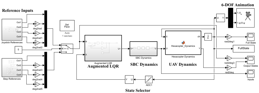
This is implemented in the MATLAB-Simulink environment while taking into account the SBC dynamics such the effects of quantisation from digital to analog and visa-versa conversions which are always present when digital controllers interface with real analog continuous-time systems.

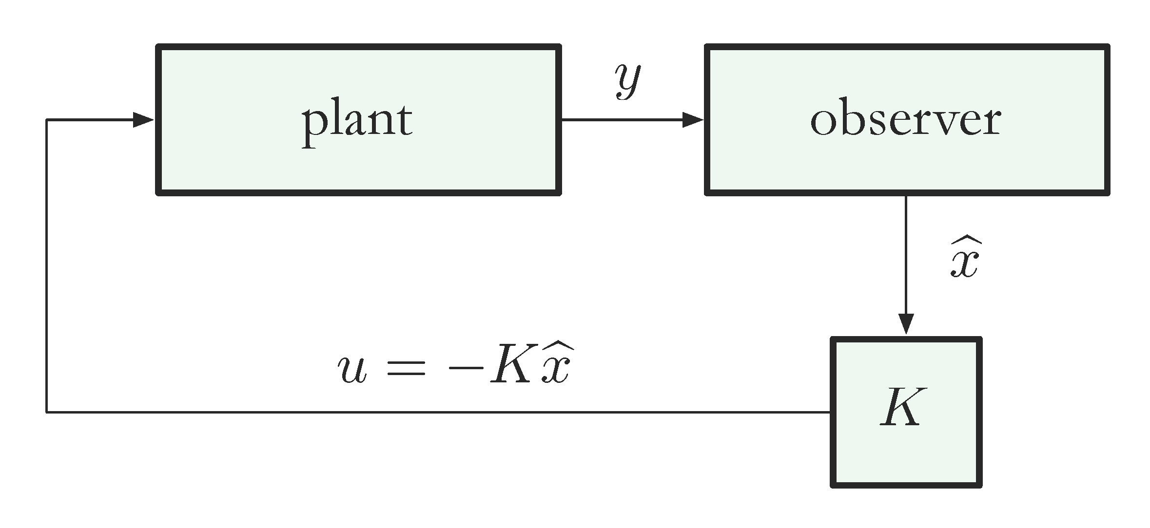
State Estimation

The control law devised in LQR subsection was produced under the assumption that the full state of the system, X, is available for full-state feedback, however, this is not the case as only a limited number of state measurements are available and these form the measured outputs, Y. Therefore, in order to utilise a full-state feedback control law, the full-state of the system must be estimated from these limited measurements present. This is performed through the implementation of a State Observer/Estimator. State estimators accomplish this by applying knowledge of the system dynamics through the utilisation of the system's model and its observability property. The estimator mimics the system dynamics giving:

$\hat{X} (k + 1) = A_{d t} \hat{X} + B_{d t} μ (k) + L e$ $\hat{Y} (k) = C_{d t} \hat{X}$

where $\hat{X}$ and $\hat{Y}$ are the estimated system states and outputs, L is the estimator gain with e being the output error, which is the difference between the estimator model and the system outputs.

$e = Y - \hat{Y}$

As with the system's model, the behaviour of estimator model and thus the quality of the estimation is determined by the state estimation error dynamics, where:

$\hat{X_{e}} = X - \hat{X}$

The open-loop estimator dynamics are given by:

$\hat{X_{e}} (k + 1) = A_{d t} (X - \hat{X})$

with implementation of the observer gain L, the closed-loop estimator dynamics are give by:

$\hat{X_{e}} (k + 1) = (A_{d t} - L C_{d t}) \hat{X_{e}}$

If the eigenvalues of the estimator exist outside the unit circle, then the estimator is unstable and the state estimation is be divergent, and if the system is observable, then it is always possible to derive some gain L, to produce any set of desired eigenvalues.

In the earlier observability subsection, it was found that the system is not observable due to propulsion unit configuration, and the emergent thrust and torque combinations making the estimation of a unique full state impossible. This can be rectified simply be making the system observable by modifying the hardware and measuring the value of some of the motor states via RPM sensors. However, there is another way this can be solved without the need to obtain additional sensors, that is, by virtually augmenting the output, Y to include terms for at least 2 out-group non coaxial motor pairs, then returning an error vector, e, where the error value for those 2 motors is 0, therefore:

$C_{y} = [\begin{matrix} 1 & 0 & 0 & 0 & 0 & 0 & 0 & 0 & 0 & 0 & 0 & 0 & 0 & 0 \\ 0 & 0 & 1 & 0 & 0 & 0 & 0 & 0 & 0 & 0 & 0 & 0 & 0 & 0 \\ 0 & 0 & 0 & 0 & 1 & 0 & 0 & 0 & 0 & 0 & 0 & 0 & 0 & 0 \\ 0 & 0 & 0 & 0 & 0 & 0 & 1 & 0 & 0 & 0 & 0 & 0 & 0 & 0 \\ 0 & 0 & 0 & 0 & 0 & 0 & 0 & 0 & 1 & 0 & 0 & 0 & 0 & 0 \\ 0 & 0 & 0 & 0 & 0 & 0 & 0 & 0 & 0 & 0 & 0 & 1 & 0 & 0 \end{matrix}], Y_{y} = [\begin{matrix} Z \\ ϕ \\ θ \\ ψ \\ ω_{1} \\ ω_{4} \end{matrix}], e = [\begin{matrix} e_{1} \\ e_{2} \\ e_{3} \\ e_{4} \\ 0 \\ 0 \end{matrix}]$

This augmentation has the effect of using the model to completely determine the value of the motor angular velocity by assuming the model is a perfect representation of the actual system. This augmentation is done solely for the purpose of state estimation so there are still only 4 reference input to the controller and only 4 measured outputs, but with this, the system is now fully observable.

Kalmam Filter

Kalman Filtering encompasses a series of techniques with a wider range of applications one such application is for obtaining an estimator gain L, which is in some wise optimal. This is accomplished by constructing an optimisation problem with the objective of minimising a set of noise measurement covariances which arise from disturbances to the system such those due to model uncertainty and noise present in the output sensor readings, these sources of noise are modelled as Gaussian noise distributions. Thus, when used in combination with the LQR, the combination is called the Linear Quadratic Gaussian. The Kalman Filter problem is a corollary problem to the LQR, where optimisation is also performed over infinite horizon, requiring the application of DP, and is thus derived resulting in another DARE. There are 2 major implementations of the Kalman filter which are popularly employed:

The Linear Kalman Filter (LKF)
The Extended Kalman Filter (EKF)

The process described above only fully pertains to the design of an LKF. The EKF is used in estimating the states of non-linear systems, utilising the non-linear system model directly but then implementing an online lineariser that linearises the system at each time interval, k, to produce a linear model which is then used to solve for the estimator gain L as stated above. There is another kalman filter implementation known as the Unscented Kalman Filter (UKF), which utilised a different linearisation technigue to the EKF, but that isnt considered here. Through experimentation with the estimator model, it was found that the systems states could be estimated by modifying the LKF to use the non linear model derived in chapter 3, similar to the EKF. This modified LKF would then use the linear model to derive the estimator gain L and the full state estimations would be derived from applying this gain to the discretised non-linear model.

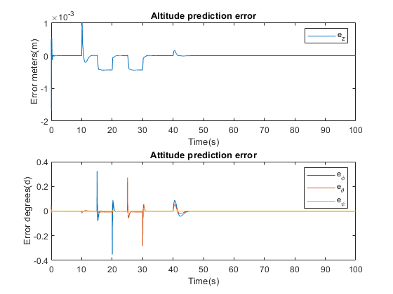
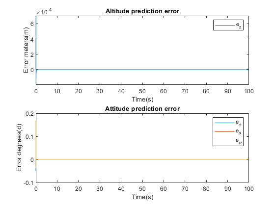
This is possible due to the limited operational scope where the system is not expected to deviate far enough from the equilibrium operating points about which the non-linear model was linearised as presented in the post on modelling. Therefore this method could be called a Limited EKF of sorts without the online linearisation. This Limited EKF modification results in more accurate state and output predictions than the standard LKF implementation, as shown when the errors between the non-linear model outputs and estimator outputs are compared.

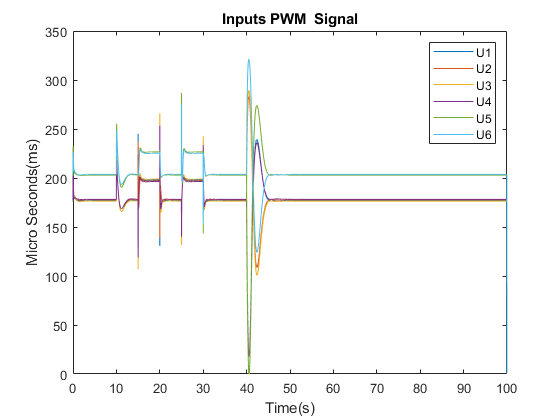
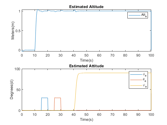
LQG Results

After Implementation of the LQG controller, all the closed-loop system eigenvalues are now within the unit circle, thus stabilising the system. Response plots of the system inputs, and the estimated, with Limited EKF, outputs of the system when subjected to reference step inputs are shown as the simulation is run over an interval of 100 seconds.