This project is taken from and is an extention of my master's dissertation which can be found here

Mathematical Modelling of Y-6 UAV

Mathematical models are used to describes the characteristics of physical systems. They are derived from assumptions made about the system which are represented abstractly. In modelling systems, it is necessary to state all assumptions made which allows for a mapping of a multirotor's movements and behaviour with the respect to its inputs and any external influences thus deriving a series of functions that map inputs onto outputs while determining all the important time dependant elements of the system. In order to successfully accomplish the development of an appropriate mathematical model for both simulation and control design, the following topics will be explored:

Kinematics
Kinetics
Actuator Dynamics
Linearisation

Multirotors can be defined as rigid-bodies free to move in 3-D space with Six Degree of Freedom, 6-DOF, with all motion restricted to being either rotational or translational. This project will derive and present 2 models, a non-linear model utilised in simulation, and a Linear model utilised in analysis and control design.

Kinematics

Multirotor mathematical models have to describe attitude and position according to the geometry of the UAV. one of the most important parts of multirotor modelling is understanding the geometric kinematic relationships between the reference frames. Kinematics is the study of motion in terms of positions and velocities without regard to the forces causing the motion. Multirotor motion can be described by a number of variables called states, that are related and change with suitably chosen axes systems or reference frames. These reference frames are:

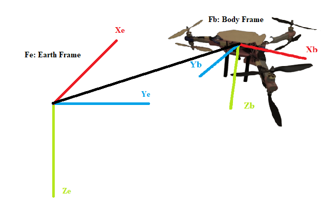
The Earth Frame: Fe
The Body Frame: Fb

Each frame consists of 3 orthogonal axes, Xe,Ye,Ze and Xb,Yb,Zb respectively, about and along which rotational and translational motion respectively occurs. Fe is fixed to the earth near the multirotor, and Fb is attached to the vehicle centred at the UAV’s centre of mass. The usual convention for the axes representation is to have an axes system with the positive Z axes pointing downwards towards the earth when level, the positive X axis pointing forward and the positive y axis pointing towards the right. This convention is referred to as the NORTH-EAST-DOWN Right-handed coordinate system.

we define state vectors:

i \begin{equation} \vec{El} = \begin{bmatrix} x \\ y \\ z \end{bmatrix} \end{equation}	ii \begin{equation} \vec{Er} = \begin{bmatrix} \phi \\ \theta \\ \psi \end{bmatrix} \end{equation}	iii \begin{equation} \vec{Bl} = \begin{bmatrix} u \\ v \\ w \end{bmatrix} \end{equation}	iv \begin{equation} \vec{Br} = \begin{bmatrix} p \\ q \\ r \end{bmatrix} \end{equation}
i Represents the linear positions of Fb’s centre with respect to (w.r.t) Fe.	ii Represents the angular rotation of Fb about all 3 axes, w.r.t Fe.(roll, pitch, yaw)	iii Represents the linear velocity in each Fb axis.	iv Represents the angular velocity in each Fb axis.

Using the $\phi, \theta, \psi$ representation, the rotational motions of Fb w.r.t Fe can be derived by looking at rotations about each axis individually. any arbitrary rotation and orientation in 3-D Euclidean space can be represented in this manner. These elemental rotation angles are known as Euler angles where rotations are represented as direction cosine matrices, These are:

\begin{equation} R_\psi = \begin{bmatrix} C_\psi & S_\psi & 0 \\ -S_\psi & C_\psi & 0 \\ 0 & 0 & 1 \end{bmatrix} \end{equation}

\begin{equation} R_\theta = \begin{bmatrix} C_\theta & 0 & -S_\theta \\ 0 & 1 & 0 \\ S_\theta & 0 & C_\theta \end{bmatrix} \end{equation}

\begin{equation} R_\phi = \begin{bmatrix} 1 & 0 & 0 \\ 0 & C_\phi & S_\phi \\ 0 & -S_\phi & C_\phi \end{bmatrix} \end{equation}

These elemental rotations can by combined via the ZYX convention to produce a matrix, the inverse of which, R, is able to map the linear velocities and accelerations in Fb to linear velocities and accelerations with respect to Fe given any set of arbitrary $\phi, \theta, \psi$ values.

\begin{equation} R = \begin{bmatrix} C_\theta C_\psi & -C_\theta S_\psi + S_\phi S_\theta C_\psi & -S_\phi S_\psi + C_\phi S_\theta C_\psi \\ C_\theta S_\psi & C_\phi C_\psi + S_\phi S_\theta S_\psi & -S_\phi C_\psi + C_\phi S_\theta S_\psi \\ -S_\theta & S_\phi C_\theta & C_\phi C_\theta \end{bmatrix} \end{equation}

\[ \dot{\vec{El}} = R \cdot \vec{Bl} \]

Similarly, to map the angular velocities and accelerations in Fb w.r.t Fe requires another transformation matrix, the inverse of which, T, is also derived from the manipulation of Euler angles.

\begin{equation} T = \begin{bmatrix} 1 & S_\phi T_\theta & C_\phi T_\theta \\ 0 & C_\phi & -S_\phi\\ 0 & \frac{S_\phi}{C_\theta} & \frac{C_\phi}{C_\theta} \end{bmatrix} \end{equation}

\[\dot{\vec{Er}} = T \cdot \vec{Br} \]

Where S, C, T, represent Sin, Cosine and Tan respectively.

Kinetics

Kinetics is the study of motion considering the forces and torques which cause the motion. As stated in the previous UAV subsection, this project looks at a Y6 hexarotor UAV which possesses 6 BLDC motors with propellers in a coaxial motor layout. Each motor propeller unit, or propulsion unit, produces a thrust force, the collective effect of which can be summed and lumped together as a single force F, where n denotes the motor index,. Each propulsion unit, also produces a reaction torque. When a motor turns, in overcoming air resistance, a reactive force acts on the propeller in the direction opposite to the motor's rotation which produce a torque acting on the UAV body. These torques, $\tau$, can then also be summed together, meaning:

\[\sum_{n = 1}^{n = 6}F_n\]

\[\sum_{n = 1}^{n = 6}\tau_n\]

The co-axial configuration also ensures single point torque balancing, meaning so long as all rotors pair each produce the same torque, the net reactive torque produced is zero. The translational and angular motion of the Y6 hexarotor is controlled by thrust forces and torques produced by each motor. The main thrust is the sum of all rotors thrust, and rotational movement is generated by differences in individual motor thrusts and torques. The Multirotor 6-DOF rigid body kinetics takes into account the mass, and the inertia of the body. These are described by differential equations, which are derived through the utilization of the Newton-Euler modelling convention which derives representations of systems dynamics through the application of first principles via newtons 2nd law of motion aggregating all forces and torques applied to the rigid body by its actuators and environment while observing the resultant accelerations produced. Resolving the Forces acting linearly on the UAV produces:

\begin{equation} M \begin{bmatrix} \ddot{x} \\ \ddot{y} \\ \ddot{z} \end{bmatrix} = M \begin{bmatrix} 0 \\ 0 \\ g \end{bmatrix} - \begin{bmatrix} C_\theta C_\psi & -C_\theta S_\psi + S_\phi S_\theta C_\psi & -S_\phi S_\psi + C_\phi S_\theta C_\psi \\ C_\theta S_\psi & C_\phi C_\psi + S_\phi S_\theta S_\psi & -S_\phi C_\psi + C_\phi S_\theta S_\psi \\ -S_\theta & S_\phi C_\theta & C_\phi C_\theta \end{bmatrix} \begin{bmatrix} 0 \\ 0 \\ \sum_{n = 1}^{n = 6}F_n \end{bmatrix} - \begin{bmatrix} D_lxx & 0 & 0 \\ 0 & D_1yy & 0 \\ 0 & 0 & D_lzz \end{bmatrix} \begin{bmatrix} \dot{x} \\ \dot{y} \\ \dot{z} \end{bmatrix} \end{equation} \[ M \cdot \ddot{\vec{El}} = M \cdot \vec{g} - M \cdot R \cdot \ddot{\vec{Bl}} - diag(D_l) \cdot \dot{\vec{El}}\]

Resolving the torques and forces acting angularly on the UAV in Fb produces:

\begin{equation} \begin{bmatrix} Ixx & 0 & 0 \\ 0 & Iyy & 0 \\ 0 & 0 & Izz \end{bmatrix} \begin{bmatrix} \dot{p} \\ \dot{q} \\ \dot{r} \end{bmatrix} = \begin{bmatrix} A_p \\ A_q \\ A_r \end{bmatrix} - \begin{bmatrix} p \\ q \\ r \end{bmatrix} \times \begin{bmatrix} Ixx & 0 & 0 \\ 0 & Iyy & 0 \\ 0 & 0 & Iyy \end{bmatrix} \begin{bmatrix} p \\ q \\ r \end{bmatrix} - \begin{bmatrix} D_rxx & 0 & 0 \\ 0 & D_ryy & 0 \\ 0 & 0 & D_rzz \end{bmatrix} \begin{bmatrix} p \\ q \\ r \end{bmatrix} \end{equation} \[ I \cdot \dot{\vec{Br}} = A - C - diag(D_r) \cdot \vec{Br} \]

where M is mass, g is acceleration due to gravity acting in the vertical Ze axis plane, $D_l$ is a diagonal matrix of drag coefficients with aerodynamic drag acting directly proportional to velocity in the Fe frame, A is the vector of torques generated by the sum of motor forces and torques in each axis, C is the Corriolis matrix formed of the cross product between the angular velocity vector and the diagonal inertia Tensor I, and $D_r$ is the diagonal matrix of drag coefficients acting against motion in each axis.

The A vector breaks down to:

\begin{equation} A_p = L_1 ((F_1+F_2) - (F_3+F_4)) \end{equation}

\begin{equation} A_q = (L_2 (F_1+F_2+F_3+F_4) - L_3 (F_5+F_6)) \end{equation}

\begin{equation} A_r = \sum_{n = 1}^{n = 6}\tau_n \end{equation}

Where L is the perpendicular distance from each motor group to the centre of mass.

Asymmetry

Due to the asymmetry of the Y6 hexarotor, mass is not even distributed across the UAV frame. This creates a particular imbalance of inertia about the centre of mass, which is the centre of all rotation in Fb. This leads to a case where I has off diagonal elements. i.e:

\begin{bmatrix} Ixx & Ixy & Ixy \\ Iyx & Iyy & Iyz \\ Izx & Izy & Izz \end{bmatrix}

This creates a situation whereby Fb, is inaccurate and instead, is transposed to some other orientation, meaning rotation about the centre mass will occur in an oblong manner. To correct this, it is possible to adjust the inertia tensor by deriving some diagonalising operation such as performing an Eigenvector decomposition, this transformation will then need to be applied to all inertia dependant terms in the angular motion calculation. However, for the purpose of this project, it is possible to operate under the assumption that the system is symmetrical, as presented by a purely diagonal inertial tensor. This is due to the off-diagonal terms in the inertia matrix being far lower in magnitude than the diagonal terms themselves, meaning that the transposed reference frame does not differ too significantly from assumed symmetrical axes, thus any deviations can be reasonably neglected.

Actuator Dynamics

The thrust forces and torques acting on the multirotor UAV are primarily generated by propulsion units consisting of a BLDC motor, an ECS and propeller. In order to produce a useful and fully developed systems model, the characteristics of the propulsion units must be known. This can either be done via first principles analysis looking at the mechanical, electrical and aerodynamic properties of each individual component, before calculating and then applying the results together in series to produce a high order high fidelity model. However taking this approach in many cases is unnecessary. This is due to being able to derive a lumped parameter model, which views the sum total of all the individual components as a single system with singular dynamics. Therefore, using system response analysis and computational methods such as data fitting, it is possible via experimental systems identification to generate a lower order, minimum realisation model of sufficient fidelity. The systems identification approach involves the derivation of lumped parameter linear input-output models, between input PWM signal widths and the output angular velocity, torque and thrust forces respectively using a motor test stand, which consists of a load cell, for measuring forces and torques as well as an electronic revolutions per minute (RPM) sensor.

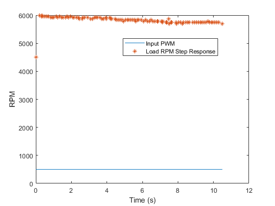
Using the Test stand, input-output PWM to RPM data is collected. the response of a propulsion unit to a step input of 500$\mu s$. This data was then passed through the MATLAB systems identification application where, in order to account for potential delays in the input response and produce a simple model, a first order transfer function was fit to the data, this transfer function can then be reformulated into a differential equation:

\[ \frac{K_u}{\tau_m s + 1} \]

\begin{equation} \dot{\omega_n} = -\frac{1}{\tau_m}\omega_n + \frac{K_u}{\tau_m}\mu_n \end{equation}

Where, $K_u$, is motor gain, $\tau_m$ is the response time constant, $\mu_n$ is the input PWM signal width and $\omega_n$ is the angular velocity. 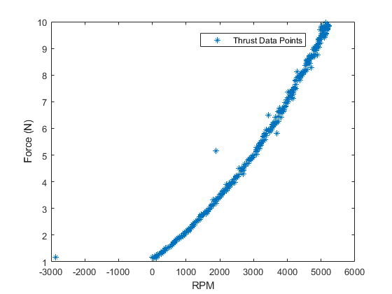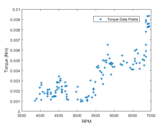The response of the identified model to the same step of 500$\mu s$.It is important to note that due to filtration present in the ESCs, the response time constant is sensitive to the frequency of the input PWM signal, therefore, throughout the investigation a frequency of 400 Hz is maintained. Similarly, using the test stand, data displaying the relationship between the force and torque produced by the propulsion unit against generated angular velocity is shown. 2 quadratic models of the form:

\begin{equation} F_n = K_a \omega_n^2 + K_b\omega_n \end{equation}

\begin{equation} \tau_n = K_\tau \omega_n^2 \end{equation}

respectively are then fit to the data where $\omega$ is the angular velocity of the motor, $K_a$, $K_b$ and $K_\tau$ are the force and torque coefficients respectively derived from the quadratic models. Due to the complex aerodynamic interactions from the overlapping air flow between the coaxial pairs, the actual thrust force produced is lower than would be expected from the sum of the two propulsion units. This loss is represented by a gain $K_w$ that is less than 1 and applied to all odd indexed propulsion units.

Non-Linear Model

Collating all the derived models process presents the following non-linear mathematical model describing the dynamics of the Y6 hexarotor UAV. which will be used to produce simulations of the system in MATLAB/Simulink.

Translational Motion:

$$ M \begin{bmatrix} \ddot{x} \\ \ddot{y} \\ \ddot{z} \end{bmatrix} = M \begin{bmatrix} 0 \\ 0 \\ g \end{bmatrix} - \begin{bmatrix} C_\theta C_\psi & -C_\theta S_\psi + S_\phi S_\theta C_\psi & -S_\phi S_\psi + C_\phi S_\theta C_\psi \\ C_\theta S_\psi & C_\phi C_\psi + S_\phi S_\theta S_\psi & -S_\phi C_\psi + C_\phi S_\theta S_\psi \\ -S_\theta & S_\phi C_\theta & C_\phi C_\theta \end{bmatrix} \begin{bmatrix} 0 \\ 0 \\ \sum F_n \end{bmatrix} - \begin{bmatrix} D_lxx & 0 & 0 \\ 0 & D_1yy & 0 \\ 0 & 0 & D_lzz \end{bmatrix} \begin{bmatrix} \dot{x} \\ \dot{y} \\ \dot{z} \end{bmatrix} $$

Rotational Motion:

$$ \begin{bmatrix} Ixx & 0 & 0 \\ 0 & Iyy & 0 \\ 0 & 0 & Izz \end{bmatrix} \begin{bmatrix} \dot{p} \\ \dot{q} \\ \dot{r} \end{bmatrix} = \begin{bmatrix} A_p \\ A_q \\ A_r \end{bmatrix} - \begin{bmatrix} p \\ q \\ r \end{bmatrix} \times \begin{bmatrix} Ixx & 0 & 0 \\ 0 & Iyy & 0 \\ 0 & 0 & Iyy \end{bmatrix} \begin{bmatrix} p \\ q \\ r \end{bmatrix} - \begin{bmatrix} D_rxx & 0 & 0 \\ 0 & D_ryy & 0 \\ 0 & 0 & D_rzz \end{bmatrix} \begin{bmatrix} p \\ q \\ r \end{bmatrix} $$

Where:

\begin{equation} A_p = L_1 ((F_1+F_2) - (F_3+F_4)) \end{equation}

\begin{equation} A_q = (L_2 (F_1+F_2+F_3+F_4) - L_3 (F_5+F_6)) \end{equation}

\begin{equation} A_r = \sum_{n = 1}^{n = 6}\tau_n \end{equation}

and motor propulsion unit dynamics are:

\[\dot{\omega_n} = -\frac{1}{\tau_m}\omega_n + \frac{K_u}{\tau_m}\mu_n\]

\[ F_n = K_a \omega_n^2 + K_b\omega_n \]

\[\tau_n = K_\tau \omega_n^2 \]

Then applying $\dot{\vec{Er}} = T \cdot \vec{Br} $ to convert angular velocity in Fb to angular velocity w.r.t Fe:

\begin{equation} \begin{bmatrix} \dot{\phi} \\ \dot{\theta} \\ \dot{\psi} \end{bmatrix} = \begin{bmatrix} 1 & S_\phi T_\theta & C_\phi T_\theta \\ 0 & C_\phi & -S_\phi\\ 0 & \frac{S_\phi}{C_\theta} & \frac{C_\phi}{C_\theta} \end{bmatrix} \begin{bmatrix} p \\ q \\ r \end{bmatrix} \end{equation}

Linearisation

As with the UAV dynamics, the majority of real world systems are non-linear. However, the majority of techniques developed in control theory have been developed for application to and analysis of linear systems. Therefore in order to utilise these techniques it is pertinent to devise some means, of operating with Non-linear systems as if they were linear. one means of accomplishing this is through the application of the Jacobian process linearisation about specific operating or equilibrium points. First however, several assumptions need to be made to reduce the model complexity making it more amicable to linearisation.

The UAV is operating in stationary hover conditions
The effects of drag are negligible
Motor dynamics are purely quadratic

Under these assumptions:

$ \ddot{\vec{Er}} \approx \dot{\vec{Br}} $
C, D_r, and D_l = 0

This reduces the model down to:

\begin{equation} \begin{bmatrix} Ixx & 0 & 0 \\ 0 & Iyy & 0 \\ 0 & 0 & Izz \end{bmatrix} \begin{bmatrix} \ddot{\phi} \\ \ddot{\theta} \\ \ddot{\psi} \end{bmatrix} = \begin{bmatrix} L_1 ((F_1+F_2) - (F_3+F_4)) \\ (L_2(F_1+F_2+F_3+F_4) - L3 (F_5+F_6)) \\ \sum_{n = 1}^{n = 6}\tau_n \end{bmatrix} \end{equation}

\[\dot{\omega_n} = -\frac{1}{\tau_m}\omega_n + \frac{K_u}{\tau_m}\mu_n\]

\[ F_n = K_a \omega_n^2 \]

\[\tau_n = K_\tau \omega_n^2 \]

Multiplying out the matrices and collecting terms produces 6 distinct 2nd order non-linear Differential, and 1 linear differential equation representing the dynamics of each motor:

\begin{equation} \ddot{x} = \frac{\sum_{n=1}^{n=6}K_a \omega_n^2}{M}C\phi S\theta C\psi + \frac{\sum_{n=1}^{n=6}K_a \omega_n^2}{M}S\phi S\psi \end{equation} \begin{equation} \ddot{y} = \frac{\sum_{n=1}^{n=6}K_a \omega_n^2}{M}C\phi S\theta C\psi - \frac{\sum_{n=1}^{n=6}K_a \omega_n^2}{M}S\phi C\psi \end{equation} \begin{equation} \ddot{z} = g - \frac{\sum_{n=1}^{n=6}K_a \omega_n^2}{M}C\phi C\theta \end{equation} \begin{equation} \ddot{\phi} = \frac{L_1}{Ixx} ((K_a \omega_1^2+K_a \omega_2^2 +) - (K_a \omega_3^2+K_a \omega_4^2)) \end{equation} \begin{equation} \ddot{\theta} = (\frac{L_2}{Iyy}(K_a \omega_1^2+K_a \omega_2^2+K_a \omega_3^2+K_a \omega_4^2) - \frac{L3}{Iyy} (K_a \omega_5^2+K_a \omega_6^2)) \end{equation} \begin{equation} \ddot{\psi} = \frac{\sum_{n = 1}^{n = 6}K_\tau \omega_n^2}{Izz} \end{equation} \begin{equation} \dot{\omega_n} = -\frac{1}{\tau_m}\omega_n + \frac{K_u}{\tau_m}\mu_n \end{equation}

Here we can define the full state vector:

$$ X = \begin{bmatrix} x,\dot{x},y,\dot{y},z,\dot{z},\phi,\dot{\phi},\theta,\dot{\theta},\psi,\dot{\psi},\omega_1,\omega_2,\omega_3,\omega_4,\omega_5,\omega_6 \end{bmatrix} $$

However for the purposes of this project the full state isn't utilised as feedback control authority in x and y are not required to maintain a stable hover. therefore, a reduced state can be defined:

$$ X = \begin{bmatrix} z,\dot{z},\phi,\dot{\phi},\theta,\dot{\theta},\psi,\dot{\psi},\omega_1,\omega_2,\omega_3,\omega_4,\omega_5,\omega_6 \end{bmatrix} $$

In order to linearise the system equations, equilibrium points must be defined. These are the set of states and input values for which the system is stationary i.e:

\[\dot{X} = f(X_e,\mu_e) = 0\]

where f represents the systems dynamics,therefore, the following equilibrium input and state vectors can be defined:

\[ X_e = \begin{bmatrix} 1.5,0,0,0,0,0,0,0,\omega_e1,\omega_e2,\omega_e3,\omega_e4,\omega_e5,\omega_e6 \end{bmatrix} \]

\[ \mu_e = \begin{bmatrix} \mu_e1,\mu_e2,\mu_e3,\mu_e4,\mu_e5,\mu_e6 \end{bmatrix} \]

Following this, the system states are redefined in terms of deviations from these equilibrium points:

\[\bar{X} = X - X_e\]

\[\bar{\mu} = \mu - \mu_e\]

These deviation variables are then substituted back into the dynamics equations and a first order Taylor's series expansion is performed. where:

\begin{equation} \dot{\bar{X}} = f(\bar{X},\bar{\mu}) + \frac{\partial f}{\partial X}\bigg\vert_{\mu = \mu_e}^{X = X_e} + \frac{\partial f}{\partial \mu}\bigg\vert_{\mu = \mu_e}^{X = X_e} \end{equation}

\[ f(\bar{X},\bar{\mu}) = 0 \]

These differential equations approximately govern the deviation variables, and as long as they remain small, this presents a linear, time-invariant, differential equation, as the derivatives of $\bar{X}$ are now linear combinations of the deviation states and the deviation inputs, $\bar{\mu}$. Finally, the Linear Continuous-Time State-Space model emerges following:

\begin{equation} A = \frac{\partial f}{\partial X}\bigg\vert_{\mu = \mu_e}^{X = X_e}, \in R ^{n\times n} \end{equation}

\begin{equation} B = \frac{\partial f}{\partial \mu}\bigg\vert_{\mu = \mu_e}^{X = X_e} , \in R ^{n\times m} \end{equation}

Where n is the number of states, m the number of inputs, A the n-by-n dynamics matrix and B the n-by-m input matrix.

Thus:

A = \begin{equation} \begin{bmatrix} 0&1&0&0&0&0&0&0&0&0&0&0&0&0\\ 0&0&0&0&0&0&0&0&\frac{2K_a\omega_e1}{M}&\frac{2K_wK_a\omega_e2}{M}&\frac{2K_a\omega_e3}{M}&\frac{2K_wK_a\omega_e4}{M}&\frac{2K_wK_a\omega_e5}{M}&\frac{2K_wK_a\omega_e6}{M}\\ 0&0&0&1&0&0&0&0&0&0&0&0&0&0\\ 0&0&0&0&0&0&0&0&\frac{2L_1K_a\omega_e1}{Ixx}&\frac{2L_1K_wK_a\omega_e2}{Ixx}& \frac{-2L_1K_a\omega_e3}{Ixx}&\frac{-2L_1K_wK_a\omega_e4}{Ixx}&0&0\\ 0&0&0&0&0&1&0&0&0&0&0&0&0&0\\ 0&0&0&0&0&0&0&0&\frac{2L_1K_a\omega_e}{Iyy}&\frac{2L_2K_wK_a\omega_e2}{Iyy}& \frac{2L_2K_a\omega_e3}{Iyy}&\frac{2L_2K_wK_a\omega_4}{Iyy}&\frac{-2L_3K_a\omega_e5}{Iyy}&\frac{-2L_3K_wK_a\omega_e6}{Iyy}\\ 0&0&0&0&0&0&0&1&0&0&0&0&0&0\\ 0&0&0&0&0&0&0&0&\frac{-2K_\tau\omega_e1}{Izz}&\frac{2K_\tau\omega_e2}{Izz}&\frac{2K_\tau\omega_e3}{Izz}&\frac{-2K_\tau\omega_e4}{Izz}&\frac{-2K_\tau\omega_e5}{Izz}&\frac{2K_\tau\omega_e6}{Izz}\\ 0&0&0&0&0&0&0&0&\frac{-1}{\tau_m}&0&0&0&0&0\\ 0&0&0&0&0&0&0&0&0&\frac{-1}{\tau_m}&0&0&0&0\\ 0&0&0&0&0&0&0&0&0&0&\frac{-1}{\tau_m}&0&0&0\\ 0&0&0&0&0&0&0&0&0&0&0&\frac{-1}{\tau_m}&0&0\\ 0&0&0&0&0&0&0&0&0&0&0&0&\frac{-1}{\tau_m}&0\\ 0&0&0&0&0&0&0&0&0&0&0&0&0&\frac{-1}{\tau_m} \end{bmatrix} \end{equation}

B = \begin{equation} \begin{bmatrix} 0&0&0&0&0&0\\ 0&0&0&0&0&0\\ 0&0&0&0&0&0\\ 0&0&0&0&0&0\\ 0&0&0&0&0&0\\ 0&0&0&0&0&0\\ 0&0&0&0&0&0\\ 0&0&0&0&0&0\\ \frac{K_u}{\tau_m}&0&0&0&0&0\\ 0&\frac{K_u}{\tau_m}&0&0&0&0\\ 0&0&\frac{K_u}{\tau_m}&0&0&0\\ 0&0&0&\frac{K_u}{\tau_m}&0&0\\ 0&0&0&0&\frac{K_u}{\tau_m}&0\\ 0&0&0&0&0&\frac{K_u}{\tau_m} \end{bmatrix} \end{equation}

Where n = 14 and m = 6