Visual Tracking and Path Planning

This section covers the technical aspects of the vision system that was implemented in the overall system. Different options that were explored are analysed and the final design of the vision system is explained in this section. The vision system comprises of 2 main components:

• Object Recognition Algorithm
• Path Planning

Requirements

• The vision system shall be able to track the position and pose of all the mobile platforms on the factory floor.
• The vision system shall be able to created an updated map of the whole factory floor and detect the position of all the nodes.
• The vision system shall do the path planning for the movement of the mobile platforms from node to node and issue high level instructions that the mobile platforms will follow.
• The vision system shall be able to detect human presence in the factory and issue a stop command to the control node.
• The vision system will contribute towards the following top level requirements: Safety, Resource Management, Communication, Planning and Security.

Transport Node Tracking: HSV Filtering

The initial approach was to have 3 RGB LEDs (WS2812) with ping pong balls mounted on top in the highlighted position on the transport node. The reason to use RGB LEDs was so that the tracking would work in any lighting conditions and the ping pong balls were used to diffuse the light and to make the markers bigger for easier tracking. Unfortunately, that didn’t work mainly because of the camera that was being used. The light from the LEDs would saturate the camera, turning them into white spots on the image regardless of the camera settings or the brightness of the LEDs. This made the system very unreliable. Ultimately, the decision to use passive markers instead of the RGB LEDs was made.

To implement the vision system, the algorithm below was implement in Python using opencv.

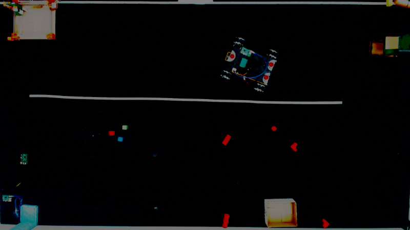
1 The image is first acquired by the camera.

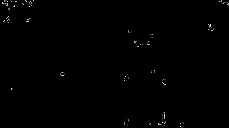
2 The HSV filtering is then applied along with the erosion and dilation.

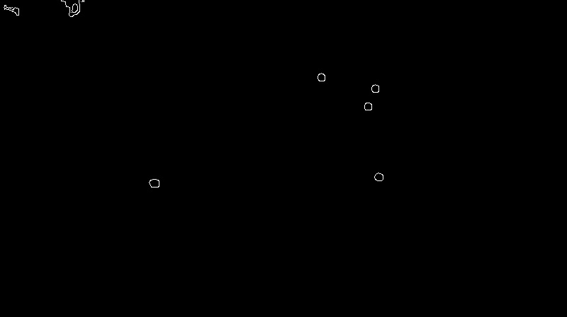
3 The size filtering is applied next.

4 From the centroid of the blobs detected, the pattern recognition algorithm is run and any 3 points conforming to the triangular geometry of the markers on the mobile platform are detected. Should any platform be detected in the arena, its pose and position are calculated from the 3 detected points.

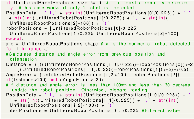
5 In order to make the tracking more reliable, an additional filter was added which worked as shown in the code below (The green text are comments and PositionData is the string posted onto the ROS topic):

Transport Node Path Planning: A* Search Algorithm

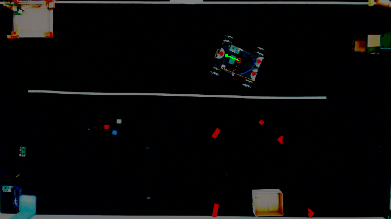
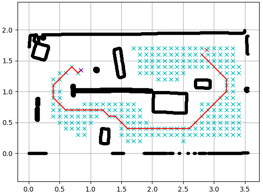
In terms of path planning, A* Search algorithm was implemented. Upon request from the Control Node, the Vision System generated a path and sent it onto the ROS topic. The PythonRobotics library by Atsushi Sakai was modified and used for the system. A path generated by the vision system is shown below:

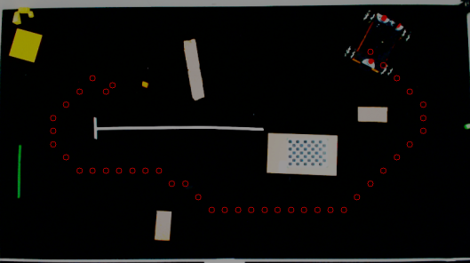
The black lines show the edge of the obstacles detected. The red line line shows the path generated while Second figure shows the points in the generated path on the original image from the camera. These coordinates are then sent on to the relevant ROS topic from where the Transport Node acquires the data and starts moving with position feedback from vision system.

The A* Search algorithm is an expression of Discrete Feasible Planning.

A Discrete feasible planning model is defined using state-space models, The basic idea is that each distinct situation for the world is called a state, denoted by x, and the set of all possible states is called a state space, X. For discrete planning, it will be important that this set is countable; in most cases it will be finite. Thus in this case, a finite state space is mapped unto the arena image captured. This state space consists of nodes at each discrete state, and edges connecting them. This is known as a graph representation.

Suppose that every edge, e ∈ E, in the graph representation of a discrete planning problem has an associated nonnegative cost l(e), which is the cost to apply some action from that state. The cost l(e) could be written using the state-space representation as l(x, u), indicating that it costs l(x, u) to apply action u from current state, x. The total cost of a plan is just the sum of the edge costs over the path from the initial state to a goal state. The cost to go from any initial state, xI, to any x is called the cost-to-come, C(x). This cost is obtained by summing edge costs, l(e), over all possible state chanages, known as paths, from the intial to the goal state, xG, and using the path that produces the least cumulative cost while storing these states in a prority queue, Q. This Process is known as Dijkstra’s algorithm.

The A∗ search algorithm is an extension of Dijkstra’s algorithm that tries to reduce the total number of states explored by incorporating a heuristic estimate of the cost to get to xG, from any given x know as cost-to-go, G(x) . There is no way to know the true optimal G(x) in advance due to possible obstacles. Fortunately, in many applications it is possible to construct a reasonable underestimate of this cost. Such as by calculating the eucledian distance between x and xG. The aim is to compute an estimate that is as close as possible to the optimal cost-to-go and is also guaranteed to be no greater, Gˆ∗(x). The A∗ search algorithm works in exactly the same way as Dijkstra’s algorithm. The only difference is the function used to sort Q. In the A∗ algorithm, the sum C∗(x′) + Gˆ∗(x′) is used, implying that the priority queue is sorted by estimates of the optimal cost from xI to XG. If Gˆ∗(x) is an underestimate of the true optimal cost-to-go for all x ∈ X, the A∗ algorithm is guaranteed to find optimal plans.